Thread: Camarilla Levels
Continuing our discussion on pivot levels, we look at the Camarilla levels which is another widely followed tool.
Word ‘Camarilla’ is borrowed from Spanish. It translates to a group of confidential & private advisers of the King or person in authority.
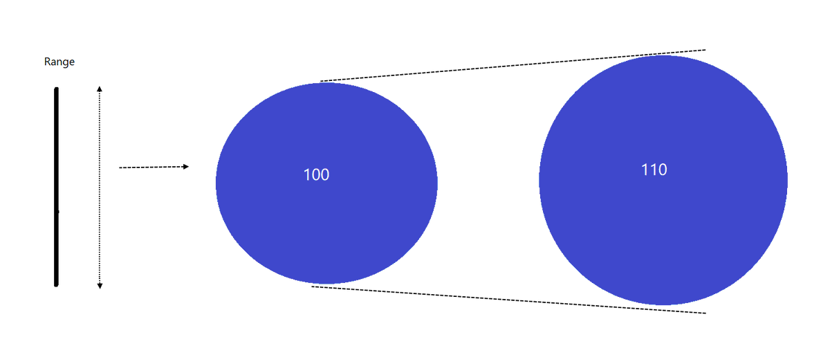
High – Low = Range of the session
Continuing with the same levels as an example, If High of the day is 105 and Low is 95, Range of the session is 10 points.
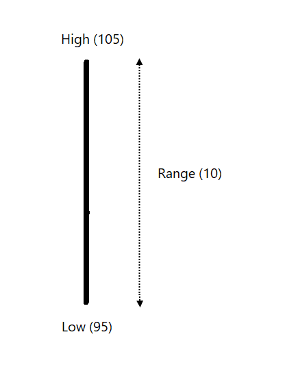
Narrow range = Not much movement
Wide Range = Strong activity
Camarilla calculation depends on the Range of the session.
Let’s expand the range to 110%. If Current range is 10, let us make it 11.
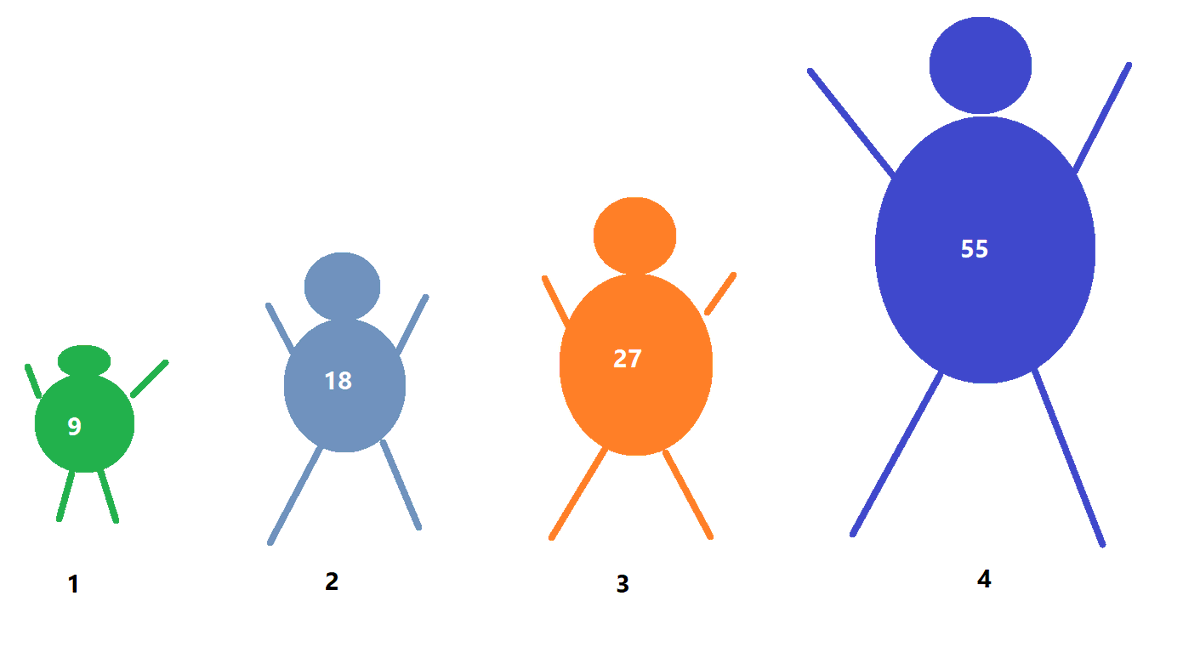
9.17%, 18.33%, 27.50% and 55% of the range.
So, if Range is 10 points:
10 x 9.17% = 0.92
10 x 18.33% = 1.83
10 x 27.50% = 2.75
10 x 55% = 5.50
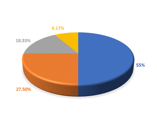
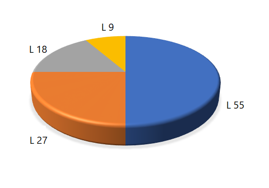
Let’s name them: L55, L27, L18 and L9.
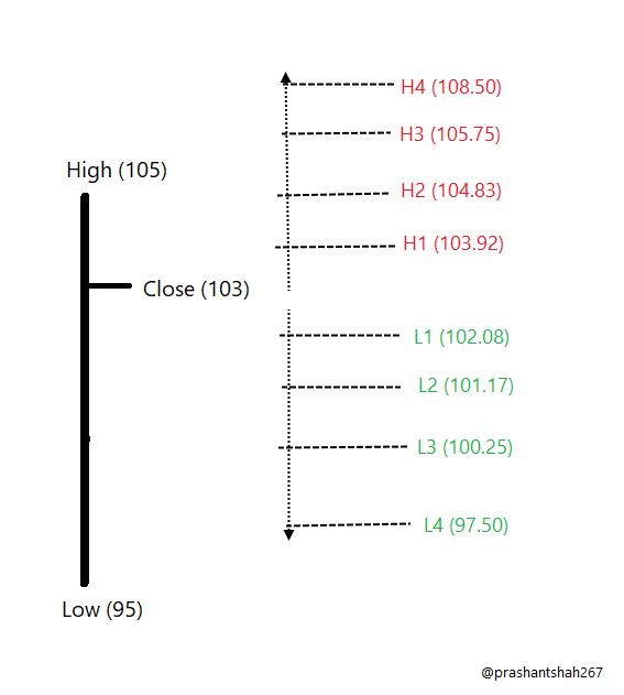
There are 8 levels in Camarilla calculation: H1, H2, H3 and H4 plotted above the close of earlier session. L1, L2, L3 and L4 plotted below the close of the earlier session.
Which factor determines the strength of bulls or bears in the session?
Close.
Range = Volatility and activity
Close = Trend and Strength
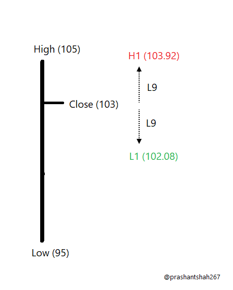
If we add L9 to the close, we get H1.
If we deduct L9 from the close, we get L1.
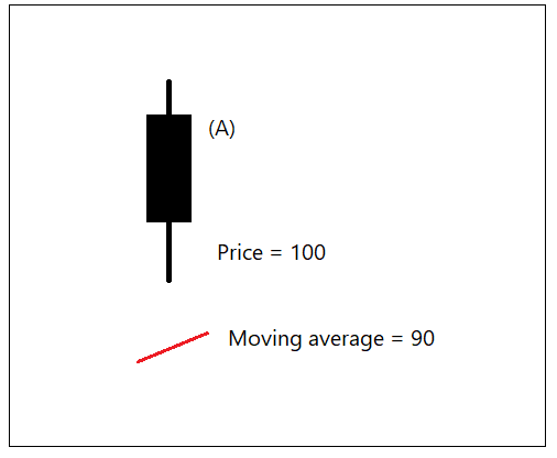
What will be H1 and L1 if High is 105, Low is 95 and Close is 103?
See the image and calculate it before reading next.
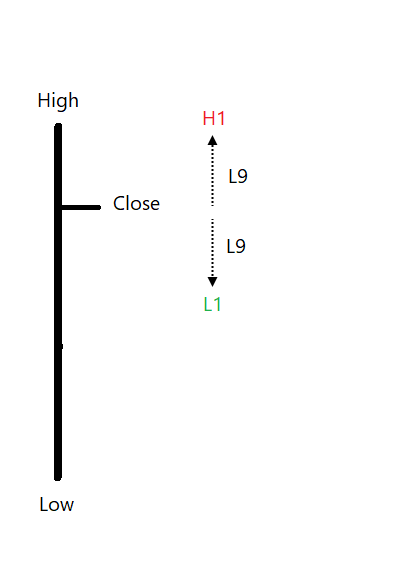
If Range is 10 points, 9.17% (L9) will be 0.92.
So,
H1 = 103.92
103 + 0.92 = 103.92
L1 = 102.08
103 – 0.92 = 102.08
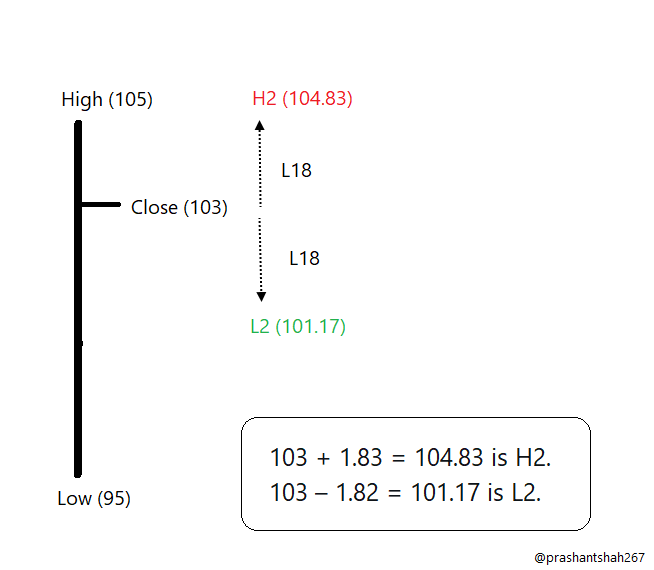
Add & deduct L18 to close to get H2 and L2.
Add & deduct L27 to close to get H3 and L3.
Add & deduct L55 to close to get H4 and L4.
Attached images explains it.
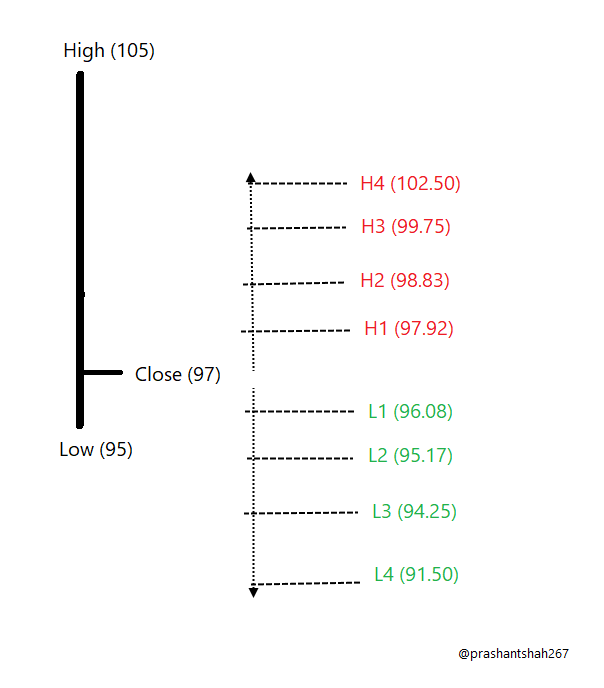
It is important to know that the position of the closing price plays an important role in placement of the levels.
Below is the calculation if closing price was 97 instead of 103.
Same range but lower levels went far from the current bar.
Hence, the next day level depends on current session trend with respect to range.
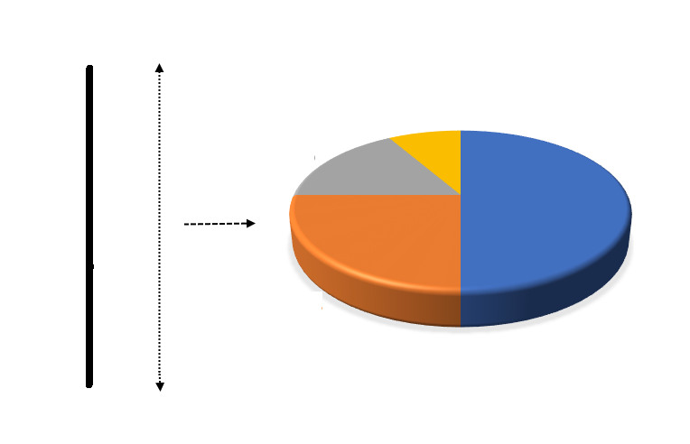
It is a simple format of distributing the range and going from lower to higher pie for referring the levels.
8.33% of the Range is first level and it expands.
8.33 -> 16.67 -> 25 -> 50
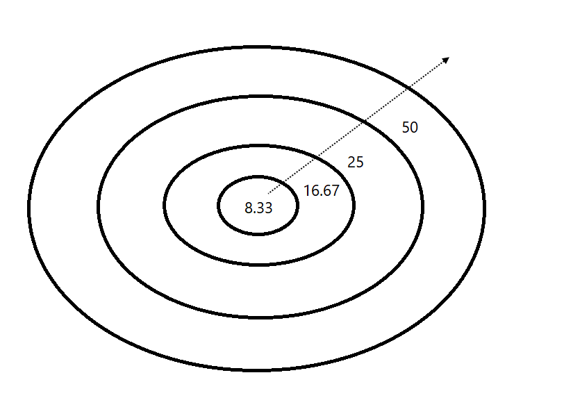
3 (L27) and 4 (L55) are strong players.
We’ll come back to the discussion on trading using these levels.
I have seen the difference in levels people use. Let's discuss them.
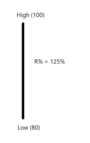
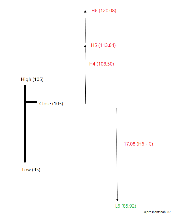
If we divide High by low price, we get the percentage of high to low. Let’s call it R%.
Eg, High is 100 & low is 80, R% is 125%.
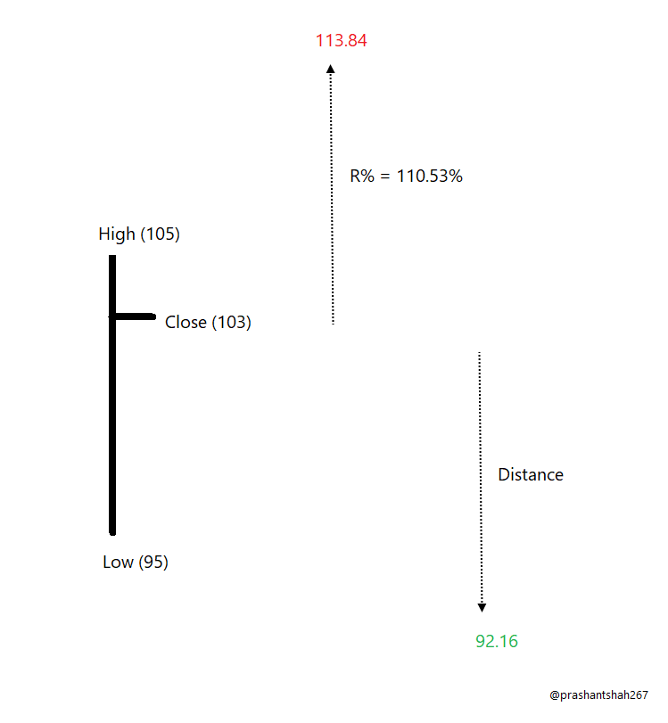
In our example, R% is 110.53% (105/95).
Close multiplied by R%
103 x 110.53% = 113.84 (RH)
Deduct distance bw close & RH to plot the equidistance lower level
103 - (113.84 – 103) = 92.16 (RL).
If the RH level is H5,
1.168 times of difference between H5 and H4 and add to H5
1.168 (113.84 – 108.50) + 113.84 = 120.08
Difference between H6 and Close to be deducted from close to get L6.
103 – 17.08 = 85.92.
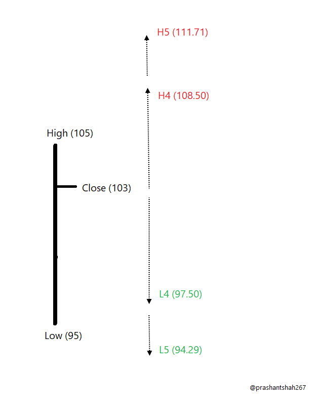
If RH is H6, 32.12% of the range is added to H4 to get H5.
10 x 32.12% = 3.21
H5
108.50 + 3.21 = 111.71
L5
97.50 – 3.21 = 94.29
I would prefer plotting R levels as H5 and L5.
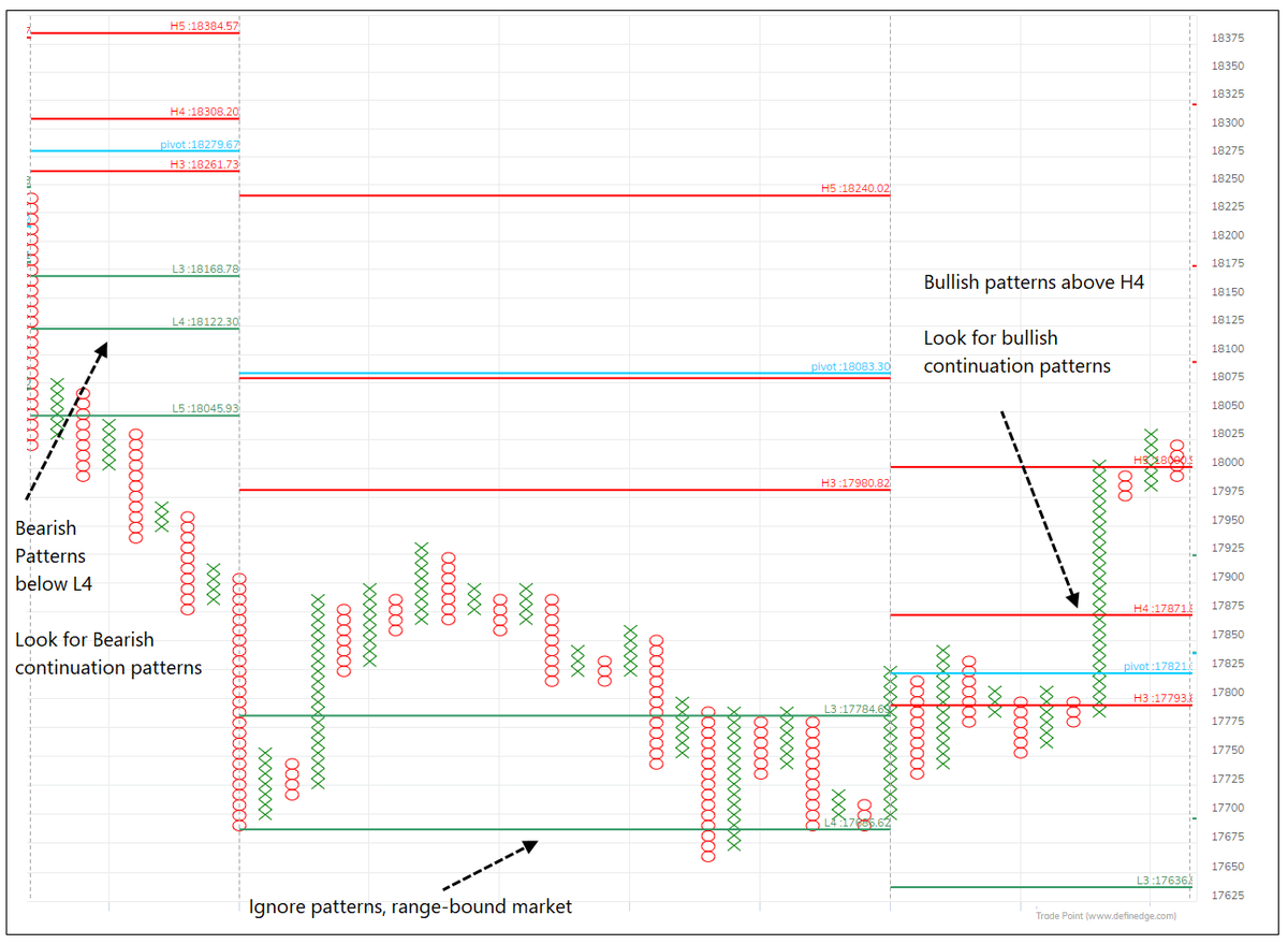
H3 and L3 are considered as mean reversion levels. They are useful in rangebound markets. Sell at H3 with stop-loss of H4, L1 and L2 are target areas. Buy at L3 with stop-loss of L4 for target areas of H1 or H2.
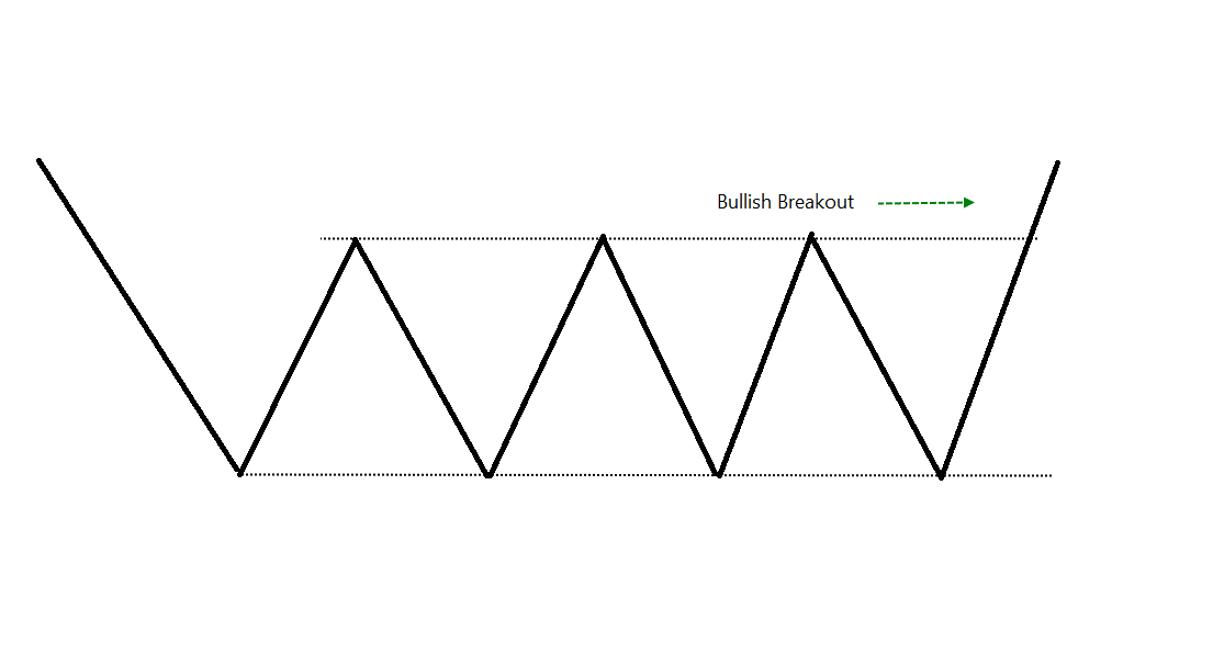
Going above H4 & falling below H3 is a bearish reversal pattern. Going below L4 & bouncing back above L3 is a bullish reversal pattern.
We can reduce it to 6.
H3 & L3 (L27) is a mean reversion.
H4 & L4 (L55) are breakout levels.
Plot R level as H5 or L5 for a target area.
So, you consider it breakout based on the highest pie of the previous range.
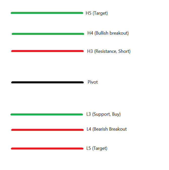
Trade breakout patterns & look for range expansion when price is beyond these levels. Else, look for mean reversion patterns or avoid trading.
Nonetheless, you can also use any of these levels for profit booking
More from Prashant Shah


You May Also Like


Fake chats claiming to be from the Irish African community are being disseminated by the far right in order to suggest that violence is imminent from #BLM supporters. This is straight out of the QAnon and Proud Boys playbook. Spread the word. Protest safely. #georgenkencho

There is co-ordination across the far right in Ireland now to stir both left and right in the hopes of creating a race war. Think critically! Fascists see the tragic killing of #georgenkencho, the grief of his community and pending investigation as a flashpoint for action.
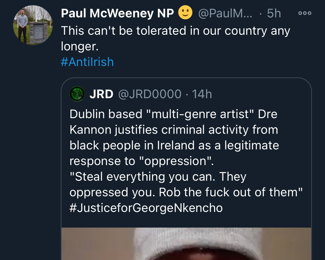
Across Telegram, Twitter and Facebook disinformation is being peddled on the back of these tragic events. From false photographs to the tactics ofwhite supremacy, the far right is clumsily trying to drive hate against minority groups and figureheads.
Declan Ganley’s Burkean group and the incel wing of National Party (Gearóid Murphy, Mick O’Keeffe & Co.) as well as all the usuals are concerted in their efforts to demonstrate their white supremacist cred. The quiet parts are today being said out loud.
The best thing you can do is challenge disinformation and report posts where engagement isn’t appropriate. Many of these are blatantly racist posts designed to drive recruitment to NP and other Nationalist groups. By all means protest but stay safe.
There is co-ordination across the far right in Ireland now to stir both left and right in the hopes of creating a race war. Think critically! Fascists see the tragic killing of #georgenkencho, the grief of his community and pending investigation as a flashpoint for action.
Across Telegram, Twitter and Facebook disinformation is being peddled on the back of these tragic events. From false photographs to the tactics ofwhite supremacy, the far right is clumsily trying to drive hate against minority groups and figureheads.
Be aware, the images the #farright are sharing in the hopes of starting a race war, are not of the SPAR employee that was punched. They\u2019re older photos of a Everton fan. Be aware of the information you\u2019re sharing and that it may be false. Always #factcheck #GeorgeNkencho pic.twitter.com/4c9w4CMk5h
— antifa.drone (@antifa_drone) December 31, 2020
Declan Ganley’s Burkean group and the incel wing of National Party (Gearóid Murphy, Mick O’Keeffe & Co.) as well as all the usuals are concerted in their efforts to demonstrate their white supremacist cred. The quiet parts are today being said out loud.
There is a concerted effort in far-right Telegram groups to try and incite violence on street by targetting people for racist online abuse following the killing of George Nkencho
— Mark Malone (@soundmigration) January 1, 2021
This follows on and is part of a misinformation campaign to polarise communities at this time.
The best thing you can do is challenge disinformation and report posts where engagement isn’t appropriate. Many of these are blatantly racist posts designed to drive recruitment to NP and other Nationalist groups. By all means protest but stay safe.