2/
A "State Quantity" is something that's associated with a *specific point in time*.
For example, the number of followers a Twitter account has is a state quantity. This number can go up and down over time. But at any one *specific* time point, it's fixed.
3/
Similarly, the amount of cash a company has is a state quantity.
This cash balance can also rise and fall over time.
But pick any one *specific* time point -- and the company can only have one *specific* cash balance at that time point.
4/
By contrast, a "Flow Quantity" is something that's associated with a time *interval* rather than a time *point*.
For example, the number of followers gained by a Twitter account is a flow quantity. It's meaningful only when we specify a time interval (eg, the last 30 days).
5/
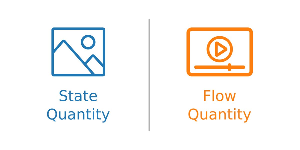
A simple analogy is that a State Quantity is like a photo -- a snapshot at a particular *point* in time.
But a Flow Quantity is like a video -- a record of events that take place during a particular time *interval*.
6/
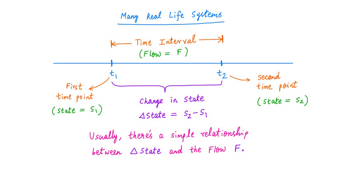
It's useful to look at many real life systems from this "State and Flow" perspective.
That's because, in many systems, the *change* in State between any 2 time points (say, t1 and t2) is usually just a simple function of the Flow during the interval (t1, t2).
7/
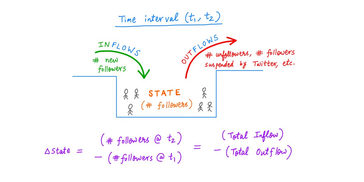
For instance, take our Twitter account example.
The State of the account at any time is the number of followers it has.
So, if we take any time interval (t1, t2), the *change* in state during this interval is simply the number of net new followers added.
8/
Logically, this must *exactly* equal Total Inflow (ie, new followers) minus Total Outflow (ie, un-followers, followers whose accounts were suspended by Twitter, etc.) during this (t1, t2) interval.
So, *change in State* exactly equals *Flow* -- our simple relationship.
9/
This may seem like a trivial example.
But many famous equations in physics, engineering, and finance are simply expressions like this -- relating "change of State" to "Flow" over some time interval.
10/
For example, the famous "Work Energy Theorem" in physics is just that.
An object's Kinetic Energy is a *State* quantity.
Work done on the object -- by applying a force to it and thereby getting it to move a certain distance -- is a *Flow* quantity.
11/
The Work Energy Theorem simply states that, during any time interval, the change in an object's Kinetic Energy must equal the Work done on it by the various forces acting on it.
See? Change in State = Flow.
12/
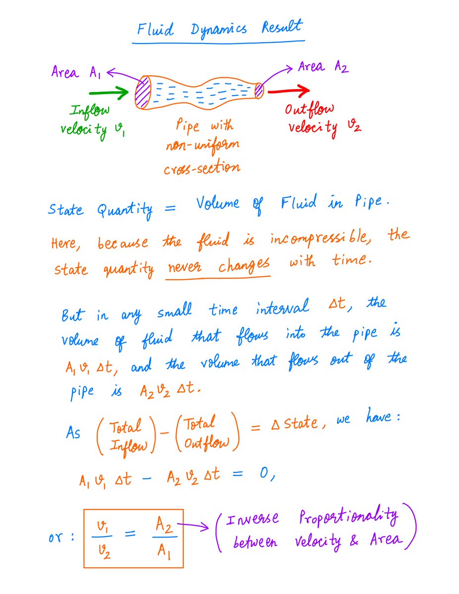
Another example is this famous result from fluid dynamics:
When an incompressible fluid flows through a pipe with non-uniform cross-section, the fluid's velocity is inversely proportional to the pipe's area of cross-section -- at any point along the pipe.
13/
This again follows from just writing out the relationship between change in State and Flow.
Here, State is the volume of fluid in the pipe -- which never changes with time as the fluid is incompressible. And Flow is the volume of fluid flowing in and out of the pipe.
14/
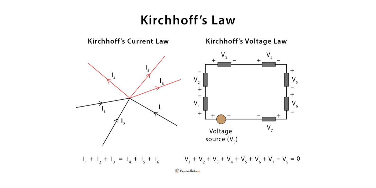
Similarly, in Electrical Engineering, voltage and charge are State quantities, whereas current is a Flow quantity.
The famous Kirchoff's voltage and current laws of circuit analysis are direct consequences of this State vs Flow perspective.
15/
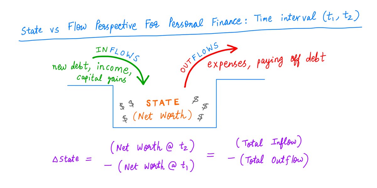
A State vs Flow perspective is also useful in finance and investing.
For example, in our personal finances, if our State is our net worth (total assets minus total liabilities) and our Flows are our incomes and expenses, we get the following:
16/
Similarly, when investing in public companies, we typically have access to 3 kinds of financial statements:
1. Balance Sheet,
2. Income Statement, and
3. Cash Flow Statement.
17/
Of these, the balance sheet is a snapshot of the company's assets and liabilities at a specific time point -- usually, the end of a quarter or year.
So, everything on the balance sheet is a State Quantity.
18/
By contrast, the income and cash flow statements are records of inflows (eg, revenues, operating cash flows) and outflows (eg, costs, increases in inventory) during a time *interval* -- usually, a quarter or year.
So, these statements are full of Flow Quantities.
19/
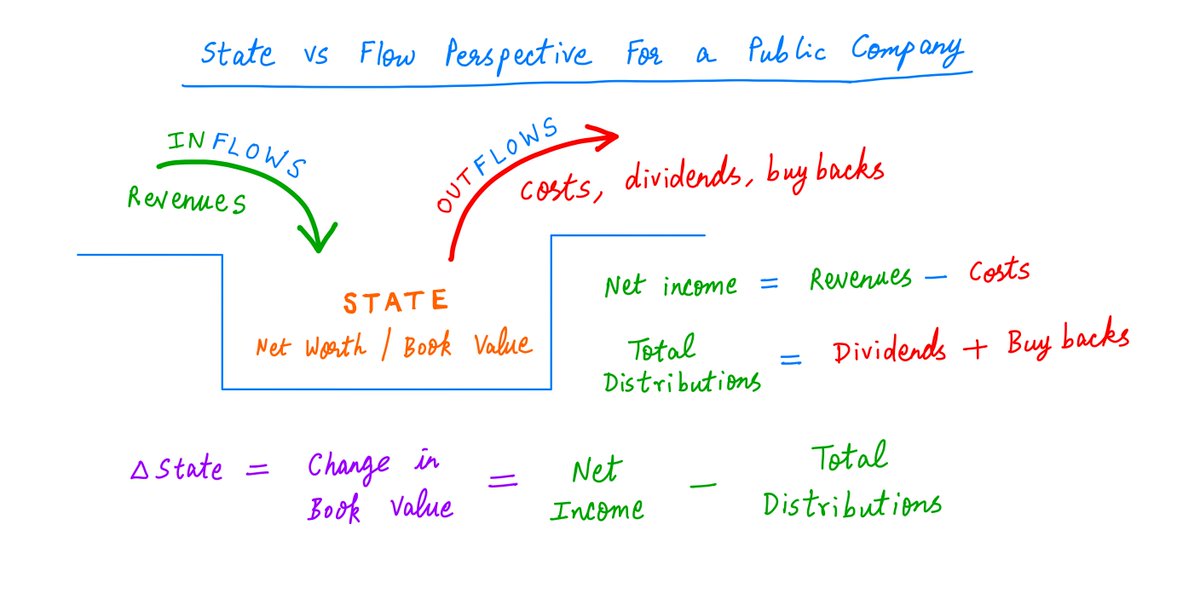
Applying our "Change of State = Flow" logic again, we see that during any quarter or year, the change in the company's net worth should be equal to its earnings (revenues minus costs) less distributions (dividends plus buybacks):
20/
Many investors use Price/Book (P/B) and Price/Earnings (P/E) ratios to value companies.
But P/B only considers a company's net worth (State).
And P/E only considers its earnings (Flow).
So, both P/B and P/E can be flawed valuation metrics.
21/
Ideally, we should value companies based on *both* State and Flow -- not just one or the other.
Also, not all earnings Flows are equal.
The *quality* of earnings matters a great deal.
22/
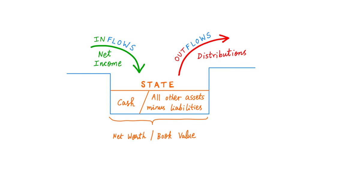
To assess the quality of earnings, it's a good idea to separate the company's net worth into 2 buckets:
Bucket 1: Cash, and
Bucket 2: All other assets, less liabilities.
23/
We separate out the company's cash because we want to study the impact of the "net income" Flow on cash specifically.
We know that net income goes to increase net worth. But net worth itself is the sum of cash and other assets.
24/
If most of net income just goes to increase "other assets" (not "cash"), then earnings are likely low quality.
For example, this happens when most of net income just shows up as an increase in working capital (inventory/receivables); this cannot be distributed to owners!
25/
But on the other hand, if most of net income goes to increase *cash*, then the earnings may be high quality -- as the cash can actually be distributed to owners via dividends and/or buybacks.
26/
But here too, there's a caveat.
"High quality earnings" means the company should be able to distribute the cash to shareholders *without hurting future earnings*.
27/
If most of the earnings are generated as cash, but then this cash has to be reinvested back into the business (or the company will lose profitability or market share!), then the earnings are not really distributable. This is just another form of low quality earnings.
28/
This need to consider *future* earnings Flows makes our State/Flow analysis a bit more complicated.
The analysis usually has 4 parts.
First, we split our State into two buckets: cash and other.
29/
Second, we work out the impact of our earnings Flows on each bucket separately -- to assess earnings quality.
High quality means lots of cash generation.
30/
Third, we try to work out how much of the cash generated needs to be reinvested back into the business just to stay in place. This "compulsory reinvestment" is called "maintenance capex".
High quality earnings means minimal maintenance capex.
31/
Fourth, we consider "growth capex".
This is cash that *can* be distributed to owners, but isn't.
Instead, it's reinvested back into the business, to grow future earnings Flows. The higher the growth per dollar of growth capex, the better the business quality.
32/
Thus, adopting a "State vs Flow" perspective can help investors understand a key feedback loop underlying most companies:
Earnings Flows produce changes in "Cash" and "Other Assets" States. Growth and maintenance capex in turn change *future* earnings Flows.
33/
Thank you very much for your kind attention!
And best wishes for a happy, healthy, and prosperous 2021.
/End
CORRECTION:
In tweet 15 above, the “new debt” inflow and “paying off debt” outflow in the picture shouldn’t be there. It’s true these are *cash* inflows and outflows, but they’re *net worth neutral* and so don’t belong in that picture. Sorry!