2/
Recently, I watched 2 probability "mini-lectures" on YouTube by Nassim Taleb.
One ~10 min lecture covered SD and MAD. The other ~6 min lecture covered Fat Tails.
In these ~16 mins,
@nntaleb shared so many useful nuggets that I had to write this thread to unpack them.
3/
For those curious, here are the YouTube links to the lectures:
SD and MAD (~10 min):
https://t.co/0TwubymdE6 Fat Tails (~6 min):
https://t.co/OoPnJLjPBN
4/
The first thing to understand is the concept of a Random Variable.
In essence, a Random Variable is a number that depends on a random event.
For example, when we roll a die, we get a Random Variable -- a number from the set {1, 2, 3, 4, 5, 6}.
5/
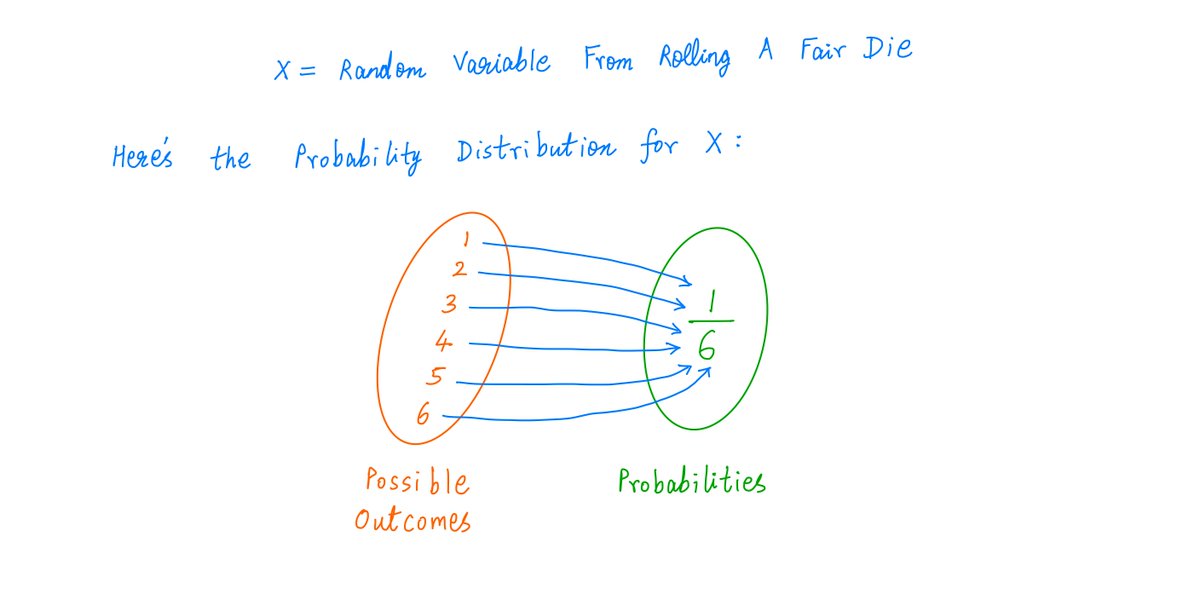
Every Random Variable has a Probability Distribution.
This tells us all the possible values the Random Variable can take, and their respective probabilities.
For example, when we roll a fair die, we get a Random Variable with this Probability Distribution:
6/
A fair die has a very simple Probability Distribution: there are only 6 possibilities, and all of them are equally likely (with probability 1/6 each).
What if our Random Variable is something more complicated?
For example, the height of a randomly chosen US adult.
7/
Now, we have more than 6 possibilities.
Any number between, say, 4 ft and 8 ft, is a possibility. There are infinitely many such numbers.
And they're not all equally likely. The extremes (4 ft, 8 ft) are rare. Most people fall in a narrow range around, say, 5.5 ft.
8/
The Gaussian Distribution is usually a good fit for this.
The average height (say, 5.5 ft) is the most likely scenario.
As we go further from the average on either side, the probabilities drop off sharply.
Like so:
9/
More precisely, the Y-axis above shows probability *densities*, not actual probabilities.
That is, we only look at height *ranges* (eg, 5 ft to 6ft), not individual heights.
For every such range, the area under the curve is the probability of lying in the range.
Like so:
10/
This is a wonderful connection between probability and geometry: we calculate probabilities by measuring areas under curves.
The total area under a probability density curve has to be 1, reflecting a 100% chance of an outcome between -infinity and +infinity.
11/
Given a distribution like this, we can ask 2 questions to try to understand it better:
First, what's the population *average*? (Also called *mean* or *expectation*, here 5.5 ft).
Second, by how much do individuals tend to *deviate* from this population mean?
12/
The first question -- calculating the population's mean -- is reasonably straightforward.
For a discrete distribution (like a die roll), we simply multiply every possible outcome by its probability, and add them all up:
13/
For a continuous distribution (like our Gaussian heights), we achieve the same thing by integrating the probability density function.
(Don't worry too much if you don't get this math.)
14/
Now for the *deviations* from the mean.
The difficulty here is that individual samples can deviate both *positively* and *negatively* from the mean.
And the way we've defined the mean guarantees that these deviations will *exactly* cancel each other out.
15/
For example, with a die roll, a 4 (deviation +0.5) exactly cancels out a 3 (deviation -0.5).
Similarly, an abnormally tall person (height 6.4 ft, deviation +0.9 ft) cancels out an abnormally short person (height 4.6 ft, deviation -0.9 ft).
16/
So, adding up these deviations gets us to a grand total of exactly zero -- no matter what the underlying probability distribution.
To get around this positive/negative cancellation, we eliminate all negative deviations -- by transforming them into positive ones.
17/
Math offers 2 simple ways to transform a negative quantity into a positive one:
- Take the *absolute value* of the negative quantity, or
- *Square* the negative quantity.
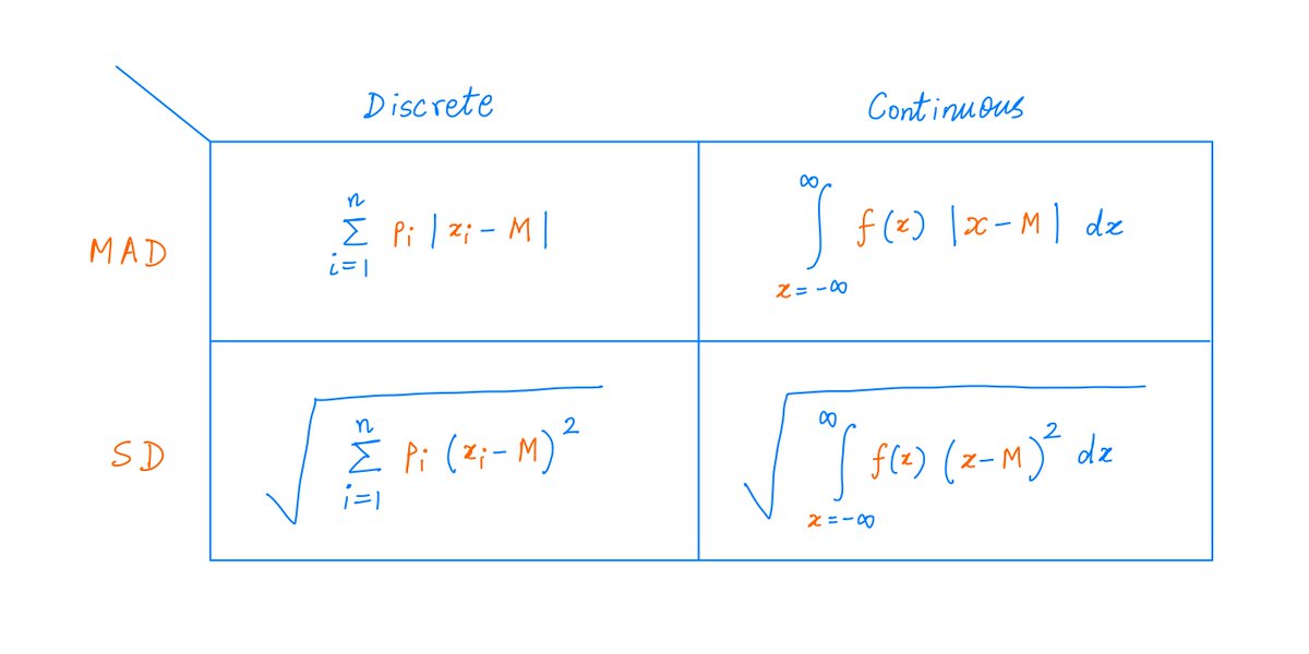
The *absolute value* leads to MAD. *Squaring* leads to SD.
Formulas:
18/
For the Gaussian Distribution, MAD and SD are given by the formulas below.
The ratio of SD to MAD is about 1.25 -- independent of the parameters mu and sigma of the distribution.
19/
So, for the Gaussian Distribution, MAD never exceeds SD.
In fact, this is a general result that follows directly from the convexity of *squaring*.
No matter what distribution we have, its MAD can never exceed its SD.
Proof:
20/
The convexity of squaring also has deeper consequences.
This is a key insight from
@nntaleb's mini-lectures.
Because squaring is convex, SD gives greater emphasis to large departures from the mean.
Such large departures, by definition, are at the tails.
21/
Therefore, SD will be much larger than MAD for Fat Tailed distributions!
In fact, the ratio of SD to MAD is an indicator of how Fat Tailed the distribution is.
For the Gaussian, this ratio is ~1.25. Not very Fat Tailed.
22/
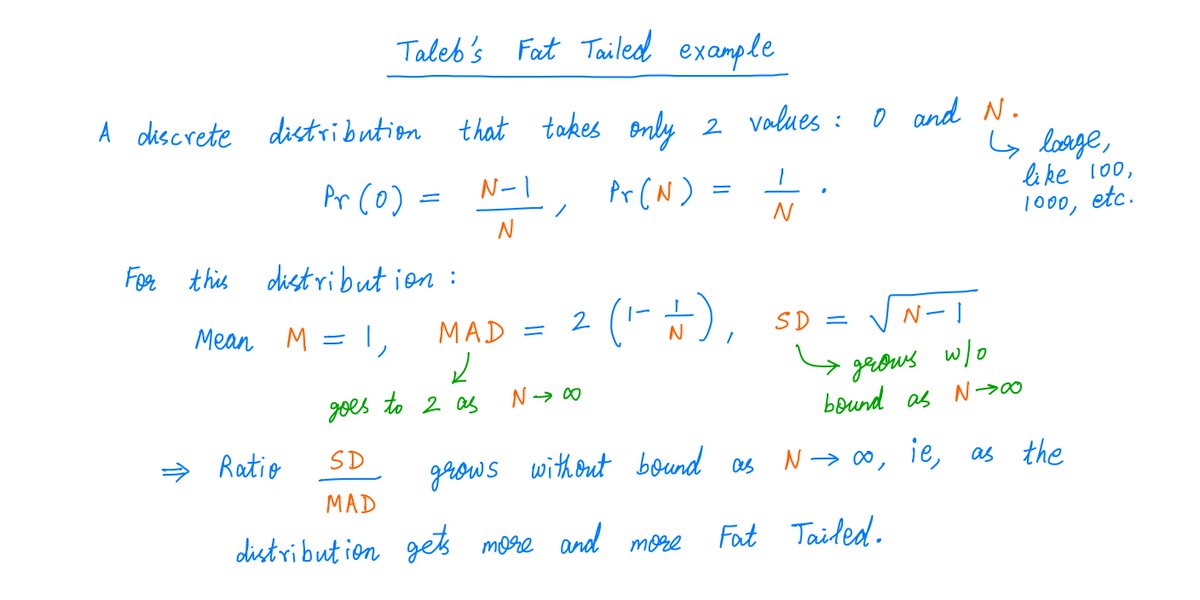
@nntaleb goes on to present a super illuminating Fat Tailed example: one large entry N in a sea of N-1 zeros.
As N gets larger, the distribution gets more and more Fat Tailed. Its SD goes to infinity. But its MAD never exceeds 2. So the SD to MAD ratio grows without bound.
23/
I had never thought about Fat Tails in terms of the "SD to MAD ratio" before. But as Taleb says, this view makes a lot of sense.
Another example of a Fat Tail is a Pareto Distribution (aka, a Power Law) -- with applications from wealth inequality to social network analysis.
24/
These distributions have 2 parameters: L and alpha.
The Random Variable can take any value greater than or equal to L, with probabilities dropping off as 1/x^(1 + alpha).
As alpha becomes larger, the Tail becomes less Fat.
The famous 80/20 Principle belongs to this class:
25/
Pareto Distributions are super interesting.
For alpha < 2, they have SD = infinity and SD/MAD = infinity! That's heavily Fat Tailed.
In particular, this applies when alpha = ~1.161, the 80/20 Principle.
Thus, SD often doesn't apply to Fat Tails. It may not even exist!
26/
There are 2 additional lenses through which we can view MAD and SD:
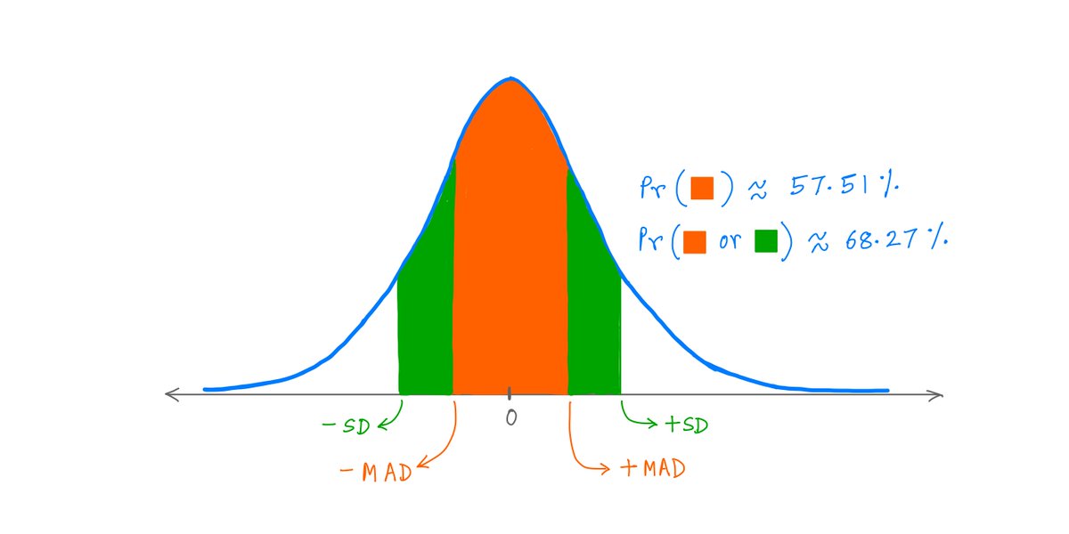
Lens 1. What % of the population lies within k deviations of the mean?
Lens 2. (Invert, Always Invert!). How many deviations are required to capture T% of the population?
27/
For example, with a Gaussian Distribution, ~57.5% of the population falls within 1 MAD of the mean. ~68.3% of the population falls within 1 SD.
Similarly, if we want to cover 90% of the population, we need a window of ~2.06 MADs (~1.64 SDs) on either side of the mean.
28/
The Fatter the Tail, the greater the % of the population that lies within k SDs of the mean.
For example, ~68.27% of a Gaussian population lies within 1 SD of its mean.
But ~92.45% of a Pareto population (L = 1, alpha = 3) lies within 1 SD of its mean.
29/
This is another key insight from Taleb's lectures.
Fatter Tails lead to a *larger* (NOT smaller) % of the population within an SD of the mean.
The convexity of squaring increases SD, and hence the fraction of the population within an SD's throw of the mean.
30/
Key lesson: Just knowing the mean and SD of a distribution may not give us enough information to reason about it intelligently.
Depending on the underlying statistics, ~68% or ~92% of the population may lie within an SD of the mean. Very different scenarios!
31/
If you're still with me, thank you very much!
I know this thread has involved somewhat more math than usual.
But I hope you got *some* feeling for MADs, SDs, and Fat Tails out of it.
Please stay safe. Enjoy your weekend!
/End